Preparation
Introduction
During this course, we will exclusively use R for data visualization and analysis, via RStudio.
The open-source programming language R is focussed on statistics and data analysis, with several built-in options and example datasets for performing most common types of analysis. For example, we can perform a regression and plot it to show the relationship between weight and miles per gallon of the cars in the built-in mtcars dataset:
result <- lm(mpg ~ wt, data = mtcars)
plot(mpg ~ wt, data = mtcars)
abline(reg = result, lty = 2)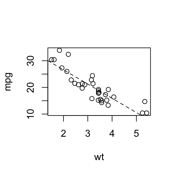
RStudio is the de-facto standard integrated development environment (IDE) for R: a computer program that enables us to easily write programs, scripts, documents, and even entire blogs, websites, and journal articles using R in the background.
We assume that you are already familiar with R and Rstudio, as outlined in the entry requirements of the course. However, if you haven’t installed R yet on your (current) computer or need some refreshing, please see below on how to install R, Rstudio and some sources to familiarize yourself with the basics.
Rstudio projects
A feature we are going to use a lot is RStudio’s projects. A project is a file folder with code, data, and other files related to a single project. An R project folder contains an .Rproj file which you can open from RStudio. This automatically sets that folder as the working directory, meaning any files in it can be loaded relative to this directory.
After opening an R project, RStudio shows the name of the project in the top-right corner of the program, above the environment panel. By clicking on it, you can close it, open another project, create new projects, and quickly access your latest projects. You can also open projects in new RStudio sessions.

R Markdown
In this course, we will make extensive use of .Rmd files, R Markdown files. With R Markdown files, we can easily create documents which seamlessly combine text, code, and plots. Even the website you are reading right now was generated from an R Markdown file.
If you’re not familiar with R Markdown files, create a new R Markdown file in RStudio using File > New File > R Markdown. Play around with the file that appears.
If you scroll through the file, you may see that there is a specific syntax associated with R Markdown files. At the start, there is some information about the document and how it should be output, and in the document itself is the text with a lot of pound signs (#), underscores (_) and backticks (\). If you are still unfamiliar with using R Markdown files, please read through the following tutorials on rmarkdown.rstudio.com before next class:
RStudio may ask you to install several packages. You should allow it to!
If these do not install, you should install and load rmarkdown; knitr and the tidyverse.
Make sure you can output the R Markdown file you created to a html using Knit > Knit to HTML on top of the source pane.
The assignments of the course need to be handed in as an R project folder with data, a .Rmd file, and the .html file generated from it.
Code style
Throughout this course, try to maintain a consistent and legible style for your code. This is very important as it will make your collaborators, as well as future you happy. Being able to read and understand your own code after a year of not looking at it is possible if you use consistent style and informative comments where necessary.
Read through the style guide on Hadley Wickham’s website.
Try to adhere to this style for your assignments, too. Tip: in RStudio, you can display a vertical line at 80 characters to know when your code exceeds this. You can do this at Tools > Global Options > Code > Display > Show margin.
R and Rstudio
1. Install R
Rcan be obtained here. We won’t useRdirectly in the course, but rather callRthroughRStudio. Therefore it needs to be installed.
2. Install RStudio Desktop
Rstudio is an Integrated Development Environment (IDE). It can be obtained as stand-alone software here. The free and open source
RStudio Desktopversion is sufficient. Also ensure that you have installed a TeX distribution, to do this run the following inRstudio:
  install.packages("tinytex")
  library(tinytex)
  install_tinytex()
3. Familiarize yourself with the basics.
Take a look at this video if you aren’t familiar with
RStudio. Additionally, since this is not a course on programming withRrather a course on data analysis and visualization, you should ensure you are familiar with some basics. For such basics you should check out:
- The first two chapters of introduction to R on datacamp
- Simply installing
R, playing around and reading Workflow basics in Hadley Wickham’s R for Data Science Book. - Interactive R Course: Install
R, and in the console type the following lines one by one:
  install.packages("swirl")
  library(swirl)
swirl()- And follow the guide to run the
R Programming: The basics of Programming in Rinteractive course.
What if the steps above do not work for me? If all fails and you have insufficient rights to your machine, the following web-based service will offer a solution.
1. Open a free account on rstudio.cloud. You can run your own cloud-based RStudio environment there.
2. Use Utrecht University’s MyWorkPlace. You would have access to R and RStudio there. You may need to install packages for new sessions during the course.
Naturally, you will need internet access for these services to be accessed.