Introduction to aDAV in R
Welcome to the practicals for the course aDAV. In the practicals we will get hands-on experience with the materials in the lectures by doing exercises, programming in R, and completing assignments.
This is the first practical. In this practical, we will briefly introduce how we are going to work with R and RStudio for the remainder of the course, and get to know (some of) the datasets that we are going to work with, and refresh our knowledge on for loops. We will also do an exercise on the distinction between supervised and unsupervised learning.
Complete and hand in the questions in the section “Part 1: to be completed at home before the lab” at least 2 hours before the start of the lab.
Before starting,
- Make sure you have read and completed the preparations.
- Read through the course schedule.
Please make sure that you do not have R and RStudio installed in a folder connected to a cloud server (e.g., OneDrive or Dropbox). You are doing these practicals to get experience with the material from the lectures and to practice for the assignments.
Part 1: to be completed at home before the lab
R projects and Markdown files
We assume that you are already familiar with R and Rstudio, as outlined in the entry requirements of the course. In addition, we assume you are familiar with using Rstudio projects and R Markdown files, as outlined in the course Preparation. If you haven’t completed the course preparation tab on the website yet, please do so before next class. If you feel you still lack some R skills, there are some sources mentioned under Preparation.
- Open the file
01_R_intro_students.Rprojin RStudio and run the following code in the console. Where is the file “sometext.txt” located on your disk?
print(readLines("data/sometext.txt"))In addition, we will make extensive use of .Rmd files, R Markdown files. With R Markdown files, we can easily create documents which seamlessly combine text, code, and plots. The document you are reading right now was generated from an R Markdown file.
Under each exercise, you can insert (if not there) an R chunk and input your code there. For questions that do not need code, you can simply add your answer as text (or as a comment inside the R chunk). If you prefer, you may also work directly in a .R file for the practicals. Note that if you do this, you will still have to work with an .Rmd file for the assignments.
- Open the file
r_introduction_stu.Rmdfrom the Files pane in RStudio, and make sure you can output the R Markdown file you created to a html usingKnit > Knit to HTMLon top of the source pane.
RStudio may ask you to install several packages. You should allow it to!
If these do not install, you should install and load rmarkdown; knitr and the tidyverse.
This way we can create an HTML file from our Rmd file.
Note: The completed homework (Part 1 of the lab) has to be handed in on Black Board and will be graded (pass/fail, counting towards your grade for individual assignment). The deadline is two hours before the start of your lab. Hand-in should be a PDF file. If you know how to knit pdf files, you can hand in the knitted pdf file. However, if you have not done this before, you are advised to knit to a html file and within the html browser, ‘print’ your file as a pdf file.
You do not need to hand in anything else after the lab.
Supervised and unsupervised learning
In the lecture and reading material for this week we have seen that machine learning can be classified on the characteristics of the data and the tasks it aims to solve. A main distinction to be made is that between supervised and unsupervised learning:
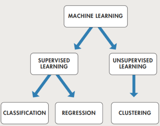
In this exercise, we will practice this distinction using 10 examples.
- Classify the following examples into Supervised learning tasks and Unsupervised learning. If they are Supervised, indicate whether a classification task or a regression task applies.
Hint: always start asking yourself if would expect a response variable in the data!
- You work at a consultancy company, and a bank hired your services. Your customer asks you to develop a model that helps them predicting which loan applicants will default (not be able to pay the loan). Final goal: predict default or non-default applicants.
- Is there a cat in the picture? Recognize cats in pictures of animals and other objects. Final goal: cat or not cat.
- A biologist friend of yours asks you to assess the phylogenetic relation between different species of birds using genetic information (traits). The outcome of your analysis is a phylogenetic tree in which species that diverged more recently are closely linked together.
 Phylogenetic tree of life built using ribosomal RNA sequences, after Karl Woese. Image credit: Modified from Eric Gaba, Wikimedia Commons.
- Using pre-existing data and satellite images containing information such as albedo, infrared refraction, colour absorption, etc., and known superficies with solar panels, train a model able of estimating the total area of solar panels per image.
- Market segmentation: group customers into segments based on their purchasing behaviours, age, maximal educational degree attained, etc.
- Predict whether nodules in a tomography are benign or malignant. You will use a dataset in which the images have been manually annotated by a committee of medic doctors.
- Use news and social media analytics to predict changes in the stock market. You will use a small number of stocks as target indicators, and web-scrapped text from social media and the news. You have access to previous instances of this data, and you want to predict the values for your indicators in the near future.
- Build a recommendation system for songs. It suggests new artists based on their multidimensional “proximity” to the ones liked by the user: “Because you liked ______ you may also like ______.”
- An applied researcher wants to evaluate whether the stress felt by students acts affects the relation between amount of study time and the probability of success on an exam . You will use a data collected in a classroom experiment.
- A pharmaceutical company is developing a drug to treat certain type of cancer. The first step is looking for targets: they ask you to analyse data consisting on the differential expression of 10,000 genes in micro-RNA chips from different tissues. You want to uncover groups of genes that display similar expression patterns in each of the tissues.
# A: Supervised learning - classification
# B: Supervised learning - classification
# C: Unsupervised learning
# D: Supervised learning - regression
# E: Unsupervised learning
# F: Supervised learning - classification
# G: Supervised learning - regression.
# H: Unsupervised learning
# I: Supervised learning. Classification (if focused on predictions, “pass or not pass”) or regression (if focused on the inference, probability estimation).
# J: Unsupervised learning- Change one of the examples above such that a supervised learning problem becomes an unsupervised learning problem or vice versa.
# We can change B to unsupervised if we are interested to group images that contain similar objects and colors.
Datasets from the ISLR package
The first book we are using in this course is Introduction to Statistical Learning, abbreviated as ISLR. The authors use several datasets throughout the book which are packaged in the R package ISLR. The datasets are: Auto, Caravan, Carseats, College, Credit, Default, Hitters, Khan, NCI60, OJ, Portfolio, Smarket, Wage, Weekly.
- Install and load the package in
Rby running the following in the console
install.packages("ISLR")
library(ISLR)
You only need to install packages once. When they are installed on your system, you can always load them in your environment using library(). Let’s have a closer look at some of the datasets we will be working with.
- Look at the Default dataset by running the following in the console. What does this dataset contain?
View(Default)# This dataset contains information for loan applicants and whehter they will default (not able to pay their loan) or not.- Look at the structure of the
Defaultdataset. Use the functionstr()to do this. What data does this dataset contain? What are the variable types?
str(Default)## 'data.frame': 10000 obs. of 4 variables:
## $ default: Factor w/ 2 levels "No","Yes": 1 1 1 1 1 1 1 1 1 1 ...
## $ student: Factor w/ 2 levels "No","Yes": 1 2 1 1 1 2 1 2 1 1 ...
## $ balance: num 730 817 1074 529 786 ...
## $ income : num 44362 12106 31767 35704 38463 ...# The dataset Default contains 10000 observations of 4 variables. The variables Balance and Income are numeric, and the variables Default and Student are of the factor type (i.e., categorical variables). - Look at the first few rows of the
Defaultdataset. Use the functionhead()to do this. Is the first observation a student or not?
head(Default)## default student balance income
## 1 No No 729.5265 44361.625
## 2 No Yes 817.1804 12106.135
## 3 No No 1073.5492 31767.139
## 4 No No 529.2506 35704.494
## 5 No No 785.6559 38463.496
## 6 No Yes 919.5885 7491.559# No, the first observation is not a studentYou made it! The rest of this lab will be completed during your lab session.
Part 2: to be completed during the lab
We hope that you have now refreshed some basic commands in R. We will continue working with some datasets and we will also work with for loops to help you refresh that as well.
- Now, let’s look at the first few rows of the
Bostondataset, contained in theMASSlibrary. What data does this dataset contain? What are the variable types? Hint: also this dataset comes with a neat help file that can be accessed through?Boston
library(MASS)##
## Attaching package: 'MASS'## The following object is masked from 'package:dplyr':
##
## selecthead(Boston)## crim zn indus chas nox rm age dis rad tax ptratio black lstat
## 1 0.00632 18 2.31 0 0.538 6.575 65.2 4.0900 1 296 15.3 396.90 4.98
## 2 0.02731 0 7.07 0 0.469 6.421 78.9 4.9671 2 242 17.8 396.90 9.14
## 3 0.02729 0 7.07 0 0.469 7.185 61.1 4.9671 2 242 17.8 392.83 4.03
## 4 0.03237 0 2.18 0 0.458 6.998 45.8 6.0622 3 222 18.7 394.63 2.94
## 5 0.06905 0 2.18 0 0.458 7.147 54.2 6.0622 3 222 18.7 396.90 5.33
## 6 0.02985 0 2.18 0 0.458 6.430 58.7 6.0622 3 222 18.7 394.12 5.21
## medv
## 1 24.0
## 2 21.6
## 3 34.7
## 4 33.4
## 5 36.2
## 6 28.7# The dataset Boston contains housing values (the variable 'medv') and other information about Boston suburbs, such as per capita crime rate. All variables are numeric (or integer, meaning numeric values without decimals). - Use the function
summary()to create a summary of theBostondataset. What is the range and median per capita crime rate by town? And what is the range of the average number of rooms per dwelling?
summary(Boston)## crim zn indus chas
## Min. : 0.00632 Min. : 0.00 Min. : 0.46 Min. :0.00000
## 1st Qu.: 0.08205 1st Qu.: 0.00 1st Qu.: 5.19 1st Qu.:0.00000
## Median : 0.25651 Median : 0.00 Median : 9.69 Median :0.00000
## Mean : 3.61352 Mean : 11.36 Mean :11.14 Mean :0.06917
## 3rd Qu.: 3.67708 3rd Qu.: 12.50 3rd Qu.:18.10 3rd Qu.:0.00000
## Max. :88.97620 Max. :100.00 Max. :27.74 Max. :1.00000
## nox rm age dis
## Min. :0.3850 Min. :3.561 Min. : 2.90 Min. : 1.130
## 1st Qu.:0.4490 1st Qu.:5.886 1st Qu.: 45.02 1st Qu.: 2.100
## Median :0.5380 Median :6.208 Median : 77.50 Median : 3.207
## Mean :0.5547 Mean :6.285 Mean : 68.57 Mean : 3.795
## 3rd Qu.:0.6240 3rd Qu.:6.623 3rd Qu.: 94.08 3rd Qu.: 5.188
## Max. :0.8710 Max. :8.780 Max. :100.00 Max. :12.127
## rad tax ptratio black
## Min. : 1.000 Min. :187.0 Min. :12.60 Min. : 0.32
## 1st Qu.: 4.000 1st Qu.:279.0 1st Qu.:17.40 1st Qu.:375.38
## Median : 5.000 Median :330.0 Median :19.05 Median :391.44
## Mean : 9.549 Mean :408.2 Mean :18.46 Mean :356.67
## 3rd Qu.:24.000 3rd Qu.:666.0 3rd Qu.:20.20 3rd Qu.:396.23
## Max. :24.000 Max. :711.0 Max. :22.00 Max. :396.90
## lstat medv
## Min. : 1.73 Min. : 5.00
## 1st Qu.: 6.95 1st Qu.:17.02
## Median :11.36 Median :21.20
## Mean :12.65 Mean :22.53
## 3rd Qu.:16.95 3rd Qu.:25.00
## Max. :37.97 Max. :50.00# The range of per captia crime rate is 0.01 - 88.98, with a median of 0.26 (hence, we have a lot of low values and only very little high values within the given range!). The average number of rooms per dwelling ranges from 3.56 to 8.78. - Let’s look at the first few rows of the
Hittersdataset. What data does this dataset contain? What are the variable types?
Hint: to get more information on what each column represents, this dataset comes with a neat help file that can be accessed through ?Hitters
head(Hitters)## AtBat Hits HmRun Runs RBI Walks Years CAtBat CHits CHmRun
## -Andy Allanson 293 66 1 30 29 14 1 293 66 1
## -Alan Ashby 315 81 7 24 38 39 14 3449 835 69
## -Alvin Davis 479 130 18 66 72 76 3 1624 457 63
## -Andre Dawson 496 141 20 65 78 37 11 5628 1575 225
## -Andres Galarraga 321 87 10 39 42 30 2 396 101 12
## -Alfredo Griffin 594 169 4 74 51 35 11 4408 1133 19
## CRuns CRBI CWalks League Division PutOuts Assists Errors
## -Andy Allanson 30 29 14 A E 446 33 20
## -Alan Ashby 321 414 375 N W 632 43 10
## -Alvin Davis 224 266 263 A W 880 82 14
## -Andre Dawson 828 838 354 N E 200 11 3
## -Andres Galarraga 48 46 33 N E 805 40 4
## -Alfredo Griffin 501 336 194 A W 282 421 25
## Salary NewLeague
## -Andy Allanson NA A
## -Alan Ashby 475.0 N
## -Alvin Davis 480.0 A
## -Andre Dawson 500.0 N
## -Andres Galarraga 91.5 N
## -Alfredo Griffin 750.0 A# The dataset Hitters contains records and salaries for baseball players. Examples of records contained are number of times at bat, hits, home runs, runs, runas batted walks and number of years in the major leages. Most of the variables are numeric (i.e., interval or ratio variables), but some variables like 'League' and 'Division' are of the factor type (i.e., categorical variables). It is also possible to select rows based on particular conditions. For example, the following code will select players that have number of home runs (HmRun) greater than 20.
runs_players <- Hitters[Hitters$HmRun > 20, ]
nrow(runs_players)
## [1] 50From the output of the code, we see that we have 50 players with home runs that is greater than 20.
- How many players are in our dataset with more than 150 hits?
high_hits_players <- Hitters[Hitters$Hits > 150, ]

nrow(high_hits_players)
## [1] 52# There are 52 players who have number of hits that is greater than 150.- Let’s now see a slightly more complicated filtering example. How many players have more 150 hits and more than 20 home runs?
hitsRunsPlayers <- Hitters[Hitters$Hits > 150 & Hitters$HmRun > 20, ]

nrow(hitsRunsPlayers)
## [1] 19# There are 19 players who have number of hits that is greater than 150 and home runs greater than 20.R Basics: For Loops
Within coding and programming for R, For Loops (or hereafter referred to as Loops) allows the repeated execution of specified commands. This is useful if you are handling a large amount of data and wish to execute the same function, adaptation or change across all/some of your data, without having to code the process line by line, which can save you significant amounts of time in the long run! For more information on Loops please see: Chapter 6 in A Beginner’s Guide to R, this Springer Textbook is a free downloadable resource which covers a huge variety of foundation topics and provided the foundation for the part below.
Conceptual Example
Lets start with a basic conceptual example (from R Bloggers), say for example you would like to print the phrase “The Year is 20XX” with XX being replaced by the years between 2010 and 2020. This could easily be achieved through writing ten individuals lines of code:
print(paste("The year is", 2010))## [1] "The year is 2010"print(paste("The year is", 2011))## [1] "The year is 2011"print(paste("The year is", 2012))## [1] "The year is 2012"print(paste("The year is", 2013))## [1] "The year is 2013"print(paste("The year is", 2014))## [1] "The year is 2014"print(paste("The year is", 2015))## [1] "The year is 2015"print(paste("The year is", 2016))## [1] "The year is 2016"print(paste("The year is", 2017))## [1] "The year is 2017"print(paste("The year is", 2018))## [1] "The year is 2018"print(paste("The year is", 2019))## [1] "The year is 2019"print(paste("The year is", 2020))## [1] "The year is 2020"Or could be written using the for() function, repeatedly executing the same command again and again.
for (year in 2010:2020){
  print(paste("The year is", year))
}
## [1] "The year is 2010"
## [1] "The year is 2011"
## [1] "The year is 2012"
## [1] "The year is 2013"
## [1] "The year is 2014"
## [1] "The year is 2015"
## [1] "The year is 2016"
## [1] "The year is 2017"
## [1] "The year is 2018"
## [1] "The year is 2019"
## [1] "The year is 2020"This basic conceptual example, is able to demonstrate to us, that the for() function is comprised clearly of two sections.
Let us consider the first section:
for (year in 2010:2020)This section contains three components:
- The function:
for(), - The parameter:
in, - The values:
year&2010:2020
Meaning as a result, these three components can be interpreted as: for value in value. Where in this case, it can be interpreted as: for year in year array.
Let us now consider the second section:
{
  print(paste("The year is", year))
}
This section is more general, and can be any function which uses the value in the for() function itself.
In this case, we can see that here year is included.
Alternatively, we can also store the year numbers in an object, and within the loop access the i’th input of the object:
year <- c(2010:2020)
for (i in 1:11){
  print(paste("The year is", year[i]))
}
## [1] "The year is 2010"
## [1] "The year is 2011"
## [1] "The year is 2012"
## [1] "The year is 2013"
## [1] "The year is 2014"
## [1] "The year is 2015"
## [1] "The year is 2016"
## [1] "The year is 2017"
## [1] "The year is 2018"
## [1] "The year is 2019"
## [1] "The year is 2020"Now let’s make our own for loop.
- Using a
loop, print the phrase ‘The month is XX’ twelve times, replacing XX by each month of the year.
month <- c("January", "February", "March", "April", "May", "June", "July", "August", "September", "October", "November", "December")

for (i in 1:12){
  print(paste("The month is", month[i]))
}
## [1] "The month is January"
## [1] "The month is February"
## [1] "The month is March"
## [1] "The month is April"
## [1] "The month is May"
## [1] "The month is June"
## [1] "The month is July"
## [1] "The month is August"
## [1] "The month is September"
## [1] "The month is October"
## [1] "The month is November"
## [1] "The month is December"Practical Example
Let us now consider a more practical example. Within the Hitters dataset, let’s say we would like to know how many of the major league players have scored a certain number of home runs. One method (although not necessarily the most straightforward) is using a loop.
for(i in Hitters$HmRun){
  print(i == 5)
}
Within this loop, we are iterating over all the values in the variable HmRun in the Hitters dataset. At each iteration, it compares the i’th observation within the dataset to the number 5, for which it then prints TRUE or FALSE depending on the result.
If you run this code, you will be able to observe the distribution in the printed values.
However: this can be seen to present as having limited value, since as the researcher you are able to only interact with this in a limited way. Instead of iterating over all values in HmRun one by one, we could also count the number of times a major league players that have a certain number of homeruns, replacing the code above by sum(Hitters$HmRun == 5). As a next step, we can use the loop to iterate over all possible number of homeruns. That is, not only inspect the exact number 5 homeruns, but all observed number of homeruns in the dataset. At this point, it becomes desirable to extend the loop to allocate the output values to a new object.
So, let us extend this previous example to count the number of times a major league player has a specific number of homeruns, and have these results saved in a separate dataframe.
HmRun.out <- data.frame(Homeruns = c(0:max(Hitters$HmRun)), Number = rep(NA, max(Hitters$HmRun) + 1))
HmRun.out
## Homeruns Number
## 1 0 NA
## 2 1 NA
## 3 2 NA
## 4 3 NA
## 5 4 NA
## 6 5 NA
## 7 6 NA
## 8 7 NA
## 9 8 NA
## 10 9 NA
## 11 10 NA
## 12 11 NA
## 13 12 NA
## 14 13 NA
## 15 14 NA
## 16 15 NA
## 17 16 NA
## 18 17 NA
## 19 18 NA
## 20 19 NA
## 21 20 NA
## 22 21 NA
## 23 22 NA
## 24 23 NA
## 25 24 NA
## 26 25 NA
## 27 26 NA
## 28 27 NA
## 29 28 NA
## 30 29 NA
## 31 30 NA
## 32 31 NA
## 33 32 NA
## 34 33 NA
## 35 34 NA
## 36 35 NA
## 37 36 NA
## 38 37 NA
## 39 38 NA
## 40 39 NA
## 41 40 NAfor(i in 0:max(Hitters$HmRun)){
HmRun.out[(i+1),2] <- sum(Hitters$HmRun == i)
}
HmRun.out## Homeruns Number
## 1 0 18
## 2 1 17
## 3 2 16
## 4 3 18
## 5 4 22
## 6 5 21
## 7 6 18
## 8 7 17
## 9 8 20
## 10 9 16
## 11 10 10
## 12 11 6
## 13 12 10
## 14 13 12
## 15 14 7
## 16 15 4
## 17 16 12
## 18 17 6
## 19 18 9
## 20 19 4
## 21 20 9
## 22 21 8
## 23 22 3
## 24 23 5
## 25 24 4
## 26 25 2
## 27 26 3
## 28 27 4
## 29 28 4
## 30 29 5
## 31 30 1
## 32 31 6
## 33 32 0
## 34 33 2
## 35 34 1
## 36 35 1
## 37 36 0
## 38 37 0
## 39 38 0
## 40 39 0
## 41 40 1For this, as you can observe the syntax itself changes, and so that for each blank unit within the empty second column of the dataframe (HmRun.out), the outcome of the statement is the number of times a specific number of homeruns was scored by a major league player. This in itself is complex, however means that you can complete this repetitive task with ease.
- Repeat the above example, but this time using a
loop, store the number of times a major league player has played a specific number of years in the major league, stored in the variableYearswithing theHittersdataset.
Years.out <- data.frame(Years = c(1:max(Hitters$Years)), Number = rep(NA, max(Hitters$Years)))
Years.out
## Years Number
## 1 1 NA
## 2 2 NA
## 3 3 NA
## 4 4 NA
## 5 5 NA
## 6 6 NA
## 7 7 NA
## 8 8 NA
## 9 9 NA
## 10 10 NA
## 11 11 NA
## 12 12 NA
## 13 13 NA
## 14 14 NA
## 15 15 NA
## 16 16 NA
## 17 17 NA
## 18 18 NA
## 19 19 NA
## 20 20 NA
## 21 21 NA
## 22 22 NA
## 23 23 NA
## 24 24 NAfor(i in 1:max(Hitters$Years)){
Years.out[i,2] <- sum(Hitters$Years == i)
}
Years.out## Years Number
## 1 1 22
## 2 2 25
## 3 3 29
## 4 4 36
## 5 5 30
## 6 6 30
## 7 7 21
## 8 8 16
## 9 9 15
## 10 10 14
## 11 11 10
## 12 12 14
## 13 13 12
## 14 14 13
## 15 15 9
## 16 16 7
## 17 17 7
## 18 18 7
## 19 19 1
## 20 20 2
## 21 21 0
## 22 22 0
## 23 23 1
## 24 24 1Code style
Throughout this course, try to maintain a consistent and legible style for your code. This is very important as it will make your collaborators, as well as future you happy. Being able to read and understand your own code after a year of not looking at it is possible if you use consistent style and informative comments where necessary.
- Read through the style guide on Hadley Wickham’s website, and name one thing you will change in your future coding endeavors after reading the style guide.
Try to adhere to this style for your assignments, too. Tip: in RStudio, you can display a vertical line at 80 characters to know when your code exceeds this. You can do this at Tools > Global Options > Code > Display > Show margin.
Conclusion
In this practical, we briefly introduced how we work with R and RStudio and we got to know (some of) the datasets that we are going to work with, and refreshed our knowledge for loops and how to style our code. We also did an exercise on the distinction between supervised and unsupervised learning.
Next week, we will have a look at the Visualization using ggplot.