Applied Data Science and Visualization > Week 3 Model accuracy and fit > Model accuracy and fit

Model accuracy and fit

Introduction

In this lab, you will learn how to plot a linear regression with confidence and prediction intervals, and various tools to assess model fit: calculating the MSE, making train-test splits, and writing a function for cross validation. You can download the student zip including all needed files for practical 3 here.

Note: the completed homework (the whole practical) has to be handed in on Black Board and will be graded (pass/fail, counting towards your grade for the individual assignment). The deadline Monday 13th of May, end of day. Hand-in should be a PDF file. If you know how to knit pdf files, you can hand in the knitted pdf file. However, if you have not done this before, you are advised to knit to a html file as specified below, and within the html browser, ‘print’ your file as a pdf file.

Please note that not all questions are dependent to each other; if you do not know the answer of one question, you can still solve part of the remaining lab.

We will use the Boston dataset, which is in the MASS package that comes with R. In addition, we will make use of the caret package to divide the Boston dataset into a training, test, and validation set.

library(ISLR)
library(MASS)
library(tidyverse)
library(caret)

As always, the first thing we want to do is to inspect the Boston dataset using the View() function:

view(Boston)

The Boston dataset contains the housing values and other information about Boston suburbs. We will use the dataset to predict housing value (the variable medv - Median value of owner-occupied homes in $1000’s - is the outcome/dependent variable) by socio-economic status (the variable lstat - % lower status of the population - is the predictor / independent variable).

Let’s explore socio-economic status and housing value in the dataset using visualization. Use the following code to create a scatter plot from the Boston dataset with lstat mapped to the x position and medv mapped to the y position. We can store the plot in an object called p_scatter.

p_scatter <- 
  Boston %>% 
  ggplot(aes(x = lstat, y = medv)) +
  geom_point() +
  theme_minimal()

p_scatter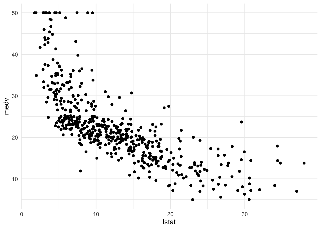

In the scatter plot, we can see that that the median value of owner-occupied homes in $1000’s (medv) is going down as the percentage of the lower status of the population (lstat) increases.

Plotting observed data including a prediction line

We’ll start with making and visualizing the linear model. As you know, a linear model is fitted in R using the function lm(), which then returns a lm object. We are going to walk through the construction of a plot with a fit line. Then we will add confidence intervals from an lm object to this plot.

First, we will create the linear model. This model will be used to predict outcomes for the current data set, and - further along in this lab - to create new data to enable adding the prediction line to the scatter plot.

Use the following code to create a linear model object called lm_ses using the formula medv ~ lstat and the Boston dataset.

lm_ses <- lm(formula = medv ~ lstat, data = Boston)

You have now trained a regression model with medv (housing value) as the outcome/dependent variable and lstat (socio-economic status) as the predictor / independent variable.

Remember that a regression estimates β (the intercept) and β₁ (the slope) in the following equation:

y = β₀ + β₁ • x₁ + ε

Use the function coef() to extract the intercept and slope from the lm_ses object. Interpret the slope coefficient.

coef(lm_ses)

## (Intercept)       lstat 
##  34.5538409  -0.9500494

# for each point increase in lstat, the median housing value drops by 0.95

Use summary() to get a summary of the lm_ses object. What do you see? You can use the help file ?summary.lm.

summary(lm_ses)

## 
## Call:
## lm(formula = medv ~ lstat, data = Boston)
## 
## Residuals:
##     Min      1Q  Median      3Q     Max 
## -15.168  -3.990  -1.318   2.034  24.500 
## 
## Coefficients:
##             Estimate Std. Error t value Pr(>|t|)    
## (Intercept) 34.55384    0.56263   61.41   <2e-16 ***
## lstat       -0.95005    0.03873  -24.53   <2e-16 ***
## ---
## Signif. codes:  0 '***' 0.001 '**' 0.01 '*' 0.05 '.' 0.1 ' ' 1
## 
## Residual standard error: 6.216 on 504 degrees of freedom
## Multiple R-squared:  0.5441,	Adjusted R-squared:  0.5432 
## F-statistic: 601.6 on 1 and 504 DF,  p-value: < 2.2e-16

We now have a model object lm_ses that represents the formula

medv_i = 34.55 - 0.95 • lstat_i + ε_i

With this object, we can predict a new medv value by inputting its lstat value. The predict() method enables us to do this for the lstat values in the original dataset.

Save the predicted y values to a variable called y_pred. Use the predict function

y_pred <- predict(lm_ses)

To generate a nice, smooth prediction line, we need a large range of (equally spaced) hypothetical lstat values. Next, we can use these hypothetical lstat values to generate predicted housing values with predict() method using the newdat argument.

One method to generate these hypothetical values is through using the function seq(). This function from base R generates a sequence of number using a standardized method. Typically length of the requested sequence divided by the range between from to to. For more information call ?seq.

Use the following code and the seq() function to generate a sequence of 1000 equally spaced values from 0 to 40. We will store this vector in a data frame with (data.frame() or tibble()) as its column name lstat. We will name the data frame pred_dat.

pred_dat <- tibble(lstat = seq(0, 40, length.out = 1000))

Now we will use the newly created data frame as the newdata argument to a predict() call for lm_ses and we will store it in a variable named y_pred_new.

y_pred_new <- predict(lm_ses, newdata = pred_dat)

Now, we’ll continue with the plotting part by adding a prediction line to the plot we previously constructed.

Use the following code to add the vector y_pred_new to the pred_dat data frame with the name medv.

# this can be done in several ways. Here are two possibilities:
# pred_dat$medv <- y_pred_new
pred_dat <- pred_dat %>% mutate(medv = y_pred_new)

Finally, we will add a geom_line() to p_scatter, with pred_dat as the data argument. What does this line represent?

p_scatter + geom_line(data = pred_dat)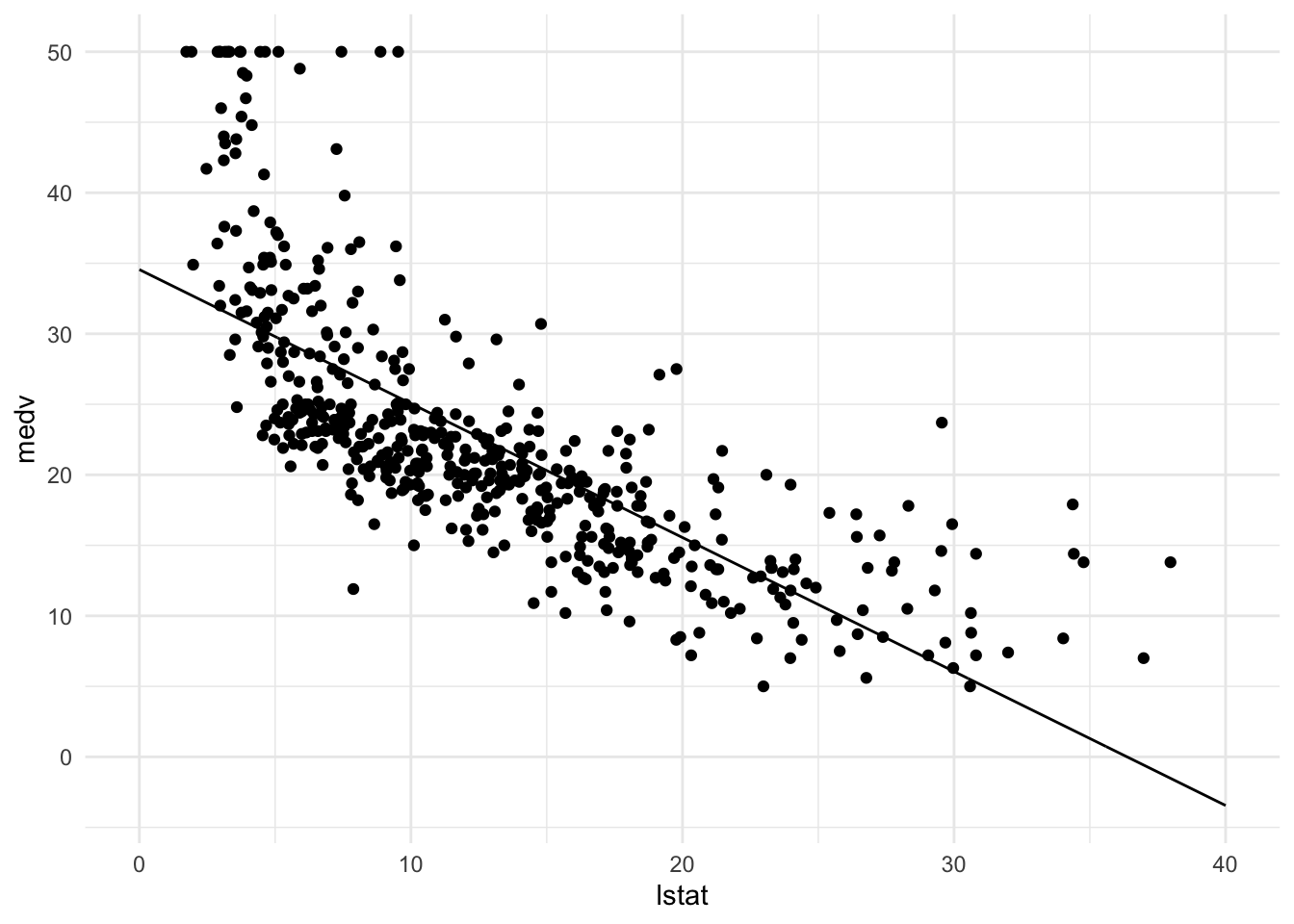

# This line represents predicted values of medv for the values of lstat

Plotting linear regression with confindence intervals

We will continue with the Boston dataset, the created model lm_ses that predicts medv (housing value) by lstat (socio-economic status), and the predicted housing values stored in y_pred. Now, we will - step by step - add confidence intervals to our plotted prediction line.

The interval argument can be used to generate confidence or prediction intervals. Create a new object called y_conf_95 using predict() (again with the pred_dat data) with the interval argument set to “confidence”. What is in this object?

y_conf_95 <- predict(lm_ses, newdata = pred_dat, interval = "confidence")

head(y_conf_95)

##        fit      lwr      upr
## 1 34.55384 33.44846 35.65922
## 2 34.51580 33.41307 35.61853
## 3 34.47776 33.37768 35.57784
## 4 34.43972 33.34229 35.53715
## 5 34.40168 33.30690 35.49646
## 6 34.36364 33.27150 35.45578

# it's a matrix with an estimate and a lower and an upper confidence interval.

Using the data from Question 5 (y_conf_95), and the sequence created earlier; create a data frame with 4 columns: medv, lstat, lower, and upper. For the lstat use the pred_dat$lstat; for medv, lower, and upper use data from y_conf_95

gg_conf <- tibble(
  lstat = pred_dat$lstat,
  medv  = y_conf_95[, 1],
  lower = y_conf_95[, 2],
  upper = y_conf_95[, 3]
)

gg_conf

## # A tibble: 1,000 × 4
##     lstat  medv lower upper
##     <dbl> <dbl> <dbl> <dbl>
##  1 0       34.6  33.4  35.7
##  2 0.0400  34.5  33.4  35.6
##  3 0.0801  34.5  33.4  35.6
##  4 0.120   34.4  33.3  35.5
##  5 0.160   34.4  33.3  35.5
##  6 0.200   34.4  33.3  35.5
##  7 0.240   34.3  33.2  35.4
##  8 0.280   34.3  33.2  35.4
##  9 0.320   34.2  33.2  35.3
## 10 0.360   34.2  33.1  35.3
## # ℹ 990 more rows

Add a geom_ribbon() to the plot with the data frame you just made. The ribbon geom requires three aesthetics: x (lstat, already mapped), ymin (lower), and ymax (upper). Add the ribbon below the geom_line() and the geom_points() of before to make sure those remain visible. Give it a nice colour and clean up the plot, too!

# Create the plot
Boston %>% 
  ggplot(aes(x = lstat, y = medv)) + 
  geom_ribbon(aes(ymin = lower, ymax = upper), data = gg_conf, fill = "#00008b44") +
  geom_point(colour = "#883321") + 
  geom_line(data = pred_dat, colour = "#00008b", size = 1) +
  theme_minimal() + 
  labs(x    = "Proportion of low SES households",
       y    = "Median house value",
       title = "Boston house prices")

## Warning: Using `size` aesthetic for lines was deprecated in ggplot2 3.4.0.
## ℹ Please use `linewidth` instead.
## This warning is displayed once every 8 hours.
## Call `lifecycle::last_lifecycle_warnings()` to see where this warning was
## generated.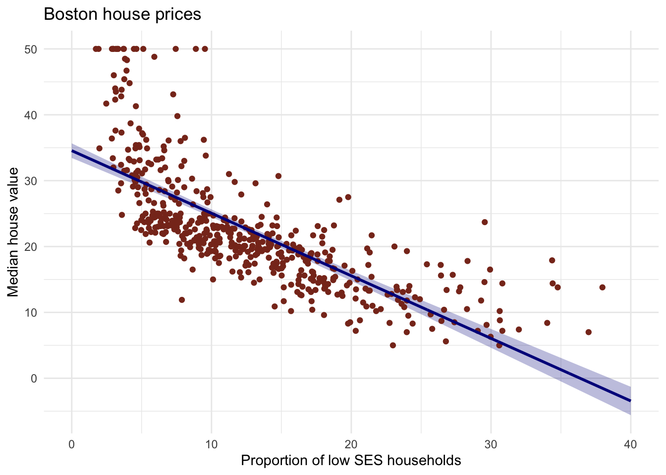

Explain in your own words what the ribbon represents.

# The ribbon represents the 95% confidence interval of the fit line.
# The uncertainty in the estimates of the coefficients are taken into
# account with this ribbon. 

# You can think of it as:
# upon repeated sampling of data from the same population, at least 95% of
# the ribbons will contain the true fit line.

Do the same thing, but now with the prediction interval instead of the confidence interval.

# pred with pred interval
y_pred_95 <- predict(lm_ses, newdata = pred_dat, interval = "prediction")


# create the df
gg_pred <- tibble(
  lstat = pred_dat$lstat,
  medv  = y_pred_95[, 1],
  l95   = y_pred_95[, 2],
  u95   = y_pred_95[, 3]
)

# Create the plot
Boston %>% 
  ggplot(aes(x = lstat, y = medv)) + 
  geom_ribbon(aes(ymin = l95, ymax = u95), data = gg_pred, fill = "#00008b44") +
  geom_point(colour = "#883321") + 
  geom_line(data = pred_dat, colour = "#00008b", size = 1) +
  theme_minimal() + 
  labs(x     = "Proportion of low SES households",
       y     = "Median house value",
       title = "Boston house prices")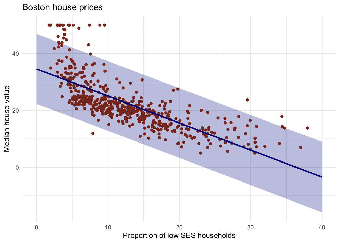

# You can look at ISLR p.81-82 for a discussion of prediction intervals

Model fit using the mean square error

Next, we will write a function to assess the model fit using the mean square error: the square of how much our predictions on average differ from the observed values. Functions are “self contained” modules of code that accomplish a specific task. Functions usually “take in” data, process it, and “return” a result. If you are not familiar with functions, please read more on chapter 19 of the book “R for Data Science” here

Write a function called mse() that takes in two vectors: true y values and predicted y values, and which outputs the mean square error.

Start like so:

mse <- function(y_true, y_pred) {
  # your formula here
}

Wikipedia may help for the formula.

# there are many ways of doing this.
mse <- function(y_true, y_pred) {
  mean((y_true - y_pred)^2)
}

Make sure your mse() function works correctly by running the following code.__

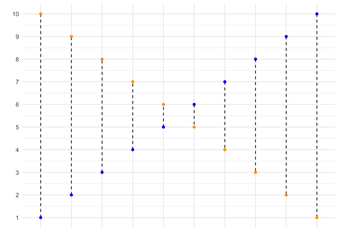
mse(1:10, 10:1)

## [1] 33

In the code, we state that our observed values correspond to $1, 2, ..., 9, 10$, while our predicted values correspond to $10, 9, ..., 2, 1$. This is graphed below, where the blue dots correspond to the observed values, and the yellow dots correspond to the predicted values. Using your function, you have now calculated the mean squared length of the dashed lines depicted in the graph below.

If your function works correctly, the value returned should equal 33.

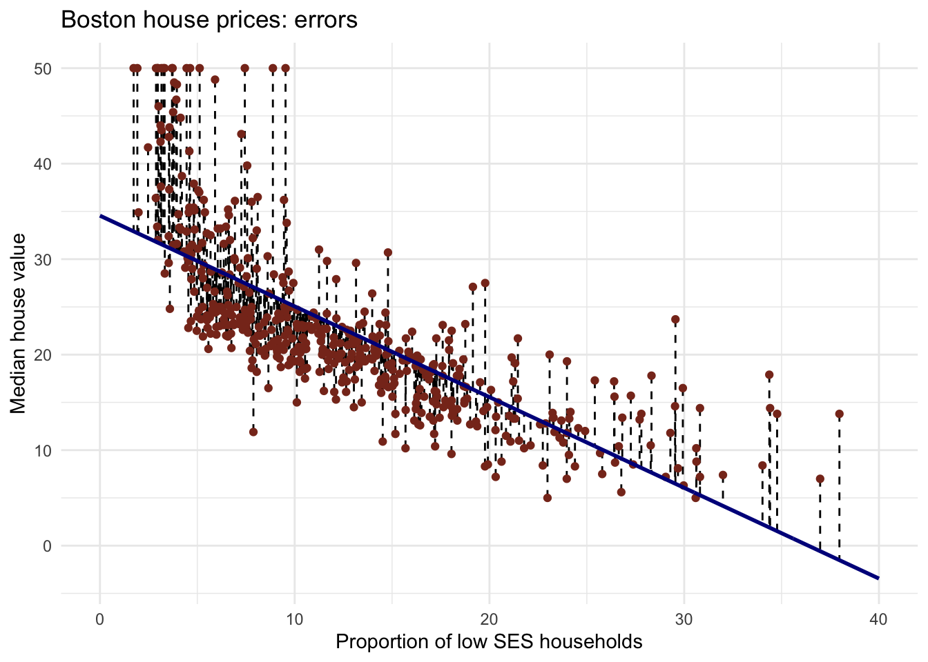
Calculate the mean square error of the lm_ses model. Use the medv column as y_true and use the predict() method to generate y_pred.

mse(Boston$medv, predict(lm_ses))

## [1] 38.48297

You have calculated the mean squared length of the dashed lines in the plot below. As the MSE is computed using the data that was used to fit the model, we actually obtained the training MSE.

Below we continue with splitting our data in a training, test and validation set such that we can calculate the out-of sample prediction error during model building using the validation set, and estimate the true out-of-sample MSE using the test set.

Note that you can also easily obtain how much the predictions on average differ from the observed values in the original scale of the outcome variable. To obtain this, you take the root of the mean square error. This is called the Root Mean Square Error, abbreviated as RMSE.

Train-validation-test splits

Next, we will use the caret package and the function createDataPartition() to obtain a training, test, and validation set from the Boston dataset. For more information on this package, see the caret website. The training set will be used to fit our model, the validation set will be used to calculate the out-of sample prediction error during model building, and the test set will be used to estimate the true out-of-sample MSE.

Use the code given below to obtain training, test, and validation set from the Boston dataset.

library(caret)
# define the training partition 
train_index <- createDataPartition(Boston$medv, p = .7, 
                                  list = FALSE, 
                                  times = 1)

# split the data using the training partition to obtain training data
boston_train <- Boston[train_index,]

# remainder of the split is the validation and test data (still) combined 
boston_val_and_test <- Boston[-train_index,]

# split the remaining 30% of the data in a validation and test set
val_index <- createDataPartition(boston_val_and_test$medv, p = .66, 
                                  list = FALSE, 
                                  times = 1)

boston_valid <- boston_val_and_test[val_index,]
boston_test  <- boston_val_and_test[-val_index,]


# Outcome of this section is that the data (100%) is split into:
# training (~70%)
# validation (~20%)
# test (~10%)

Note that creating the partitions using the y argument (letting the function know what your dependent variable will be in the analysis), makes sure that when your dependent variable is a factor, the random sampling occurs within each class and should preserve the overall class distribution of the data.

We will set aside the boston_test dataset for now.

Train a linear regression model called model_1 using the training dataset. Use the formula medv ~ lstat like in the first lm() exercise. Use summary() to check that this object is as you expect.

model_1 <- lm(medv ~ lstat, data = boston_train)
summary(model_1)

## 
## Call:
## lm(formula = medv ~ lstat, data = boston_train)
## 
## Residuals:
##     Min      1Q  Median      3Q     Max 
## -10.077  -4.069  -1.463   1.960  24.369 
## 
## Coefficients:
##             Estimate Std. Error t value Pr(>|t|)    
## (Intercept) 34.73523    0.67019   51.83   <2e-16 ***
## lstat       -0.95536    0.04615  -20.70   <2e-16 ***
## ---
## Signif. codes:  0 '***' 0.001 '**' 0.01 '*' 0.05 '.' 0.1 ' ' 1
## 
## Residual standard error: 6.314 on 354 degrees of freedom
## Multiple R-squared:  0.5476,	Adjusted R-squared:  0.5463 
## F-statistic: 428.5 on 1 and 354 DF,  p-value: < 2.2e-16

Calculate the MSE with this object. Save this value as model_1_mse_train.

model_1_mse_train <- mse(y_true = boston_train$medv, y_pred = predict(model_1))
model_1_mse_train

## [1] 39.64747

Now calculate the MSE on the validation set and assign it to variable model_1_mse_valid. Hint: use the newdata argument in predict().

model_1_mse_valid <- mse(y_true = boston_valid$medv, 
                         y_pred = predict(object = model_1, newdata = boston_valid))

This is the estimated out-of-sample mean squared error.

Create a second model model_2 for the train data which includes age and tax as predictors. Calculate the train and validation MSE.

model_2 <- lm(medv ~ lstat + age + tax, data = boston_train)
summary(model_2)

## 
## Call:
## lm(formula = medv ~ lstat + age + tax, data = boston_train)
## 
## Residuals:
##     Min      1Q  Median      3Q     Max 
## -10.279  -3.928  -1.539   1.774  24.144 
## 
## Coefficients:
##              Estimate Std. Error t value Pr(>|t|)    
## (Intercept) 34.169164   0.995308  34.330  < 2e-16 ***
## lstat       -0.993880   0.058990 -16.848  < 2e-16 ***
## age          0.044987   0.015461   2.910  0.00385 ** 
## tax         -0.005016   0.002408  -2.083  0.03801 *  
## ---
## Signif. codes:  0 '***' 0.001 '**' 0.01 '*' 0.05 '.' 0.1 ' ' 1
## 
## Residual standard error: 6.244 on 352 degrees of freedom
## Multiple R-squared:  0.5601,	Adjusted R-squared:  0.5563 
## F-statistic: 149.4 on 3 and 352 DF,  p-value: < 2.2e-16

model_2_mse_train <- mse(y_true = boston_train$medv, y_pred = predict(model_2))
model_2_mse_train

## [1] 38.55239

model_2_mse_valid <- mse(y_true = boston_valid$medv, 
                         y_pred = predict(model_2, newdata = boston_valid))

Compare model 1 and model 2 in terms of their training and validation MSE. Which would you choose and why?

# If you are interested in out-of-sample prediction, the 
# answer may depend on the random sampling of the rows in the
# dataset splitting: everyone has a different split. However, it
# is likely that model_2 has both lower training and validation MSE.

In choosing the best model, you should base your answer on the validation MSE. Using the out of sample mean square error, we have made a model decision (which parameters to include, only lstat, or using age and tax in addition to lstat to predict housing value). Now we have selected a final model.

For your final model, retrain the model one more time using both the training and the validation set. Then, calculate the test MSE based on the (retrained) final model. What does this number tell you?

model_2b <- lm(medv ~ lstat + age + tax, data = bind_rows(boston_train, boston_valid))
summary(model_2b)

## 
## Call:
## lm(formula = medv ~ lstat + age + tax, data = bind_rows(boston_train, 
##     boston_valid))
## 
## Residuals:
##     Min      1Q  Median      3Q     Max 
## -16.795  -3.877  -1.345   1.840  24.714 
## 
## Coefficients:
##              Estimate Std. Error t value Pr(>|t|)    
## (Intercept) 34.350241   0.856411  40.110  < 2e-16 ***
## lstat       -0.958201   0.052344 -18.306  < 2e-16 ***
## age          0.046908   0.013296   3.528 0.000461 ***
## tax         -0.006941   0.002077  -3.342 0.000901 ***
## ---
## Signif. codes:  0 '***' 0.001 '**' 0.01 '*' 0.05 '.' 0.1 ' ' 1
## 
## Residual standard error: 6.126 on 454 degrees of freedom
## Multiple R-squared:  0.5578,	Adjusted R-squared:  0.5549 
## F-statistic: 190.9 on 3 and 454 DF,  p-value: < 2.2e-16

model_2_mse_test <- mse(y_true = boston_test$medv, 
                        y_pred = predict(model_2b, newdata = boston_test))
model_2_mse_test

## [1] 34.43521

# The estimate for the expected amount of error when predicting 
# the median value of a not previously seen town in Boston when 
# using this model is:

sqrt(model_2_mse_test)

## [1] 5.868152

As you will see during the remainder of the course, usually we set apart the test set at the beginning and on the remaining data perform the train-validation split multiple times. Performing the train-validation split multiple times is what we for example do in cross validation (see below). The validation sets are used for making model decisions, such as selecting predictors or tuning model parameters, so building the model. As the validation set is used to base model decisions on, we can not use this set to obtain a true out-of-sample MSE. That’s where the test set comes in, it can be used to obtain the MSE of the final model that we choose when all model decisions have been made. As all model decisions have been made, we can use all data except for the test set to retrain our model one last time using as much data as possible to estimate the parameters for the final model.

Optional: cross-validation

This is an advanced exercise. Some components we have seen before in this lab, but some things will be completely new. Try to complete it by yourself, but don’t worry if you get stuck. If you need to refresh your memory on for loops in R, have another look at lab 1 on the course website.

Use help in this order:

R help files
Internet search & stack exchange
Your peers
The answer, which shows one solution

You may also just read the answer when they have been made available and try to understand what happens in each step.

Create a function that performs k-fold cross-validation for linear models.

Inputs:

formula: a formula just as in the lm() function
dataset: a data frame
k: the number of folds for cross validation
any other arguments you need necessary

Outputs:

Mean square error averaged over folds

# Just for reference, here is the mse() function once more
mse <- function(y_true, y_pred) mean((y_true - y_pred)^2)

cv_lm <- function(formula, dataset, k) {
  # We can do some error checking before starting the function
  stopifnot(is_formula(formula))       # formula must be a formula
  stopifnot(is.data.frame(dataset))    # dataset must be data frame
  stopifnot(is.integer(as.integer(k))) # k must be convertible to int
  
  # first, add a selection column to the dataset as before
  n_samples  <- nrow(dataset)
  select_vec <- rep(1:k, length.out = n_samples)
  data_split <- dataset %>% mutate(folds = sample(select_vec))
  
  # initialise an output vector of k mse values, which we 
  # will fill by using a _for loop_ going over each fold
  mses <- rep(0, k)
  
  # start the for loop
  for (i in 1:k) {
    # split the data in train and validation set
    data_train <- data_split %>% filter(folds != i)
    data_valid <- data_split %>% filter(folds == i)
    
    # calculate the model on this data
    model_i <- lm(formula = formula, data = data_train)
    
    # Extract the y column name from the formula
    y_column_name <- as.character(formula)[2]
    
    # calculate the mean square error and assign it to mses
    mses[i] <- mse(y_true = data_valid[[y_column_name]],
                   y_pred = predict(model_i, newdata = data_valid))
  }
  
  # now we have a vector of k mse values. All we need is to
  # return the mean mse!
  mean(mses)
}

Use your function to perform 9-fold cross validation with a linear model with as its formula medv ~ lstat + age + tax. Compare it to a model with as formula medv ~ lstat + I(lstat^2) + age + tax.

cv_lm(formula = medv ~ lstat + age + tax, dataset = Boston, k = 9)

## [1] 38.33556

cv_lm(formula = medv ~ lstat + I(lstat^2) + age + tax, dataset = Boston, k = 9)

## [1] 27.93643