Applied Data Science and Visualization > Week 4 Linear Regression for Data Science > Linear regression for data science

Linear regression for data science

Part 1: to be completed at home before the lab

In this lab, you will learn how to handle many variables with regression by using variable selection techniques, shrinkage techniques, and how to tune hyper-parameters for these techniques. This practical has been derived from chapter 6 of ISLR. You can download the student zip including all needed files for practical 4 here.

Note: the completed homework has to be handed in on Black Board and will be graded (pass/fail, counting towards your grade for the individual assignment). The deadline is two hours before the start of your lab. Hand-in should be a PDF or HTML file.

In addition, you will need for loops (see also lab 1), data manipulation techniques from Dplyr, and the caret package (see lab week 3) to create a training, validation and test split for the used dataset. Another package we are going to use is glmnet. For this, you will probably need to install.packages("glmnet") before running the library() functions.

library(ISLR)
library(glmnet)
library(tidyverse)
library(caret)

Best subset selection

Our goal is to to predict Salary from the Hitters dataset from the ISLR package. In this at home section, we will do the pre-work for best-subset selection. First, we will prepare a dataframe baseball from the Hitters dataset where you remove the baseball players for which the Salary is missing. Use the following code:

baseball <- Hitters %>% filter(!is.na(Salary))

We can check how many baseball players are left using:

nrow(baseball)

## [1] 263

1. a) Create baseball_train (50%), baseball_valid (30%), and baseball_test (20%) datasets using the createDataPartition() function of the caret package.

1. b) Using your knowledge of ggplot from lab 2, plot the salary information of the train, validate and test groups using geom_histogram() or geom_density()

We will use the following function which we called lm_mse() to obtain the mse on the validation dataset for predictions from a linear model:

lm_mse <- function(formula, train_data, valid_data) {
  y_name <- as.character(formula)[2]
  y_true <- valid_data[[y_name]]
  
  lm_fit <- lm(formula, train_data)
  y_pred <- predict(lm_fit, newdata = valid_data)
  
  mean((y_true - y_pred)^2)
}

Note that the input consists of (1) a formula, (2) a training dataset, and (3) a test dataset.

2. Try out the function with the formula Salary ~ Hits + Runs, using baseball_train and baseball_valid.

We have pre-programmed a function for you to generate a character vector for all formulas with a set number of p variables. You can load the function into your environment by sourcing the .R file it is written in:

source("generate_formulas.R")

You can use it like so:

generate_formulas(p = 2, x_vars = c("x1", "x2", "x3", "x4"), y_var = "y")

## [1] "y ~ x1 + x2" "y ~ x1 + x3" "y ~ x1 + x4" "y ~ x2 + x3" "y ~ x2 + x4"
## [6] "y ~ x3 + x4"

3. Create a character vector of all predictor variables from the Hitters dataset. colnames() may be of help. Note that Salary is not a predictor variable.

4. Using the function generate_formulas() (which is inlcuded in your project folder for lab week 4), generate all formulas with as outcome Salary and 3 predictors from the Hitters data. Assign this to a variable called formulas. There should be 969 elements in this vector.

5. We will use the following code to find the best set of 3 predictors in the Hitters dataset based on MSE using the baseball_train and baseball_valid datasets. Annotate the following code with comments that explain what each line is doing.

mses <- rep(0, 969)
for (i in 1:969) {
  mses[i] <- lm_mse(as.formula(formulas[i]), baseball_train, baseball_valid)
}

best_3_preds <- formulas[which.min(mses)]

6. Find the best set for 1, 2 and 4 predictors. Now select the best model from the models with the best set of 1, 2, 3, or 4 predictors in terms of its out-of-sample MSE

Part 2: to be completed during the lab

7. a) Calculate the test MSE for the model with the best number of predictors. You can first train the model with the best predictors on the combination of training and validation set and save it to a variable. Also, you will need a function that calculates the mse.

7. b) Using the model with the best number of predictors (the one you created in the previous question), create a plot comparing predicted values (mapped to x position) versus observed values (mapped to y position) of baseball_test.

Through enumerating all possibilities, we have selected the best subset of at most 4 non-interacting predictors for the prediction of baseball salaries. This method works well for few predictors, but the computational cost of enumeration increases quickly to the point where it is not feasible to enumerate all combinations of variables:

## Warning: Using `size` aesthetic for lines was deprecated in ggplot2 3.4.0.
## ℹ Please use `linewidth` instead.
## This warning is displayed once every 8 hours.
## Call `lifecycle::last_lifecycle_warnings()` to see where this warning was
## generated.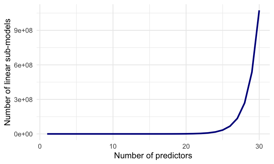

Regularization with glmnet

glmnet is a package that implements efficient (quick!) algorithms for LASSO and ridge regression, among other things.

8. Skim through the help file of glmnet. We are going to perform a linear regression with normal (gaussian) error terms. What format should our data be in?

Again, we will try to predict baseball salary, this time using all the available variables and using the LASSO penalty to perform subset selection. For this, we first need to generate an input matrix.

9. First generate the input matrix using (a variation on) the following code. Remember that the “.” in a formula means “all available variables”. Make sure to check that this x_train looks like what you would expect.

x_train <- model.matrix(Salary ~ ., data = baseball_train)

The model.matrix() function takes a dataset and a formula and outputs the predictor matrix where the categorical variables have been correctly transformed into dummy variables, and it adds an intercept. It is used internally by the lm() function as well!

10. Using glmnet(), perform a LASSO regression with the generated x_train as the predictor matrix and Salary as the response variable. Set the lambda parameter of the penalty to 15. NB: Remove the intercept column from the x_matrix – glmnet adds an intercept internally.

11. The coefficients for the variables are in the beta element of the list generated by the glmnet() function. Which variables have been selected? You may use the coef() function.

12. Now we will create a predicted versus observed plot for the baseball_valid data using the model we just generated. To do this, first generate the input matrix with the baseball_valid data. Then use the predict() function to generate the predictions for the baseball_valid data using the model matrix and the model you created in question 10. Finally, create the predicted versus observed plot for the validation data. What is the MSE on the validation set?

Tuning lambda

Like many methods of analysis, regularized regression has a tuning parameter. In the previous section, we’ve set this parameter to 15. The lambda parameter changes the strength of the shrinkage in glmnet(). Changing the tuning parameter will change the predictions, and thus the MSE. In this section, we will select the tuning parameter based on out-of-sample MSE.

13. a) Fit a LASSO regression model on the same data as before, but now do not enter a specific lambda value. What is different about the object that is generated? Hint: use the coef() and plot() methods on the resulting object.

13. b) To help you interpret the obtained plot, Google and explain the qualitative relationship between L1 norm (the maximum allowed sum of coefs) and lambda.

For deciding which value of lambda to choose, we could work similarly to what we have don in the best subset selection section before. However, the glmnet package includes another method for this task: cross validation.

14. Use the cv.glmnet function to determine the lambda value for which the out-of-sample MSE is lowest using 15-fold cross validation. As your dataset, you may use the training and validation sets bound together with bind_rows(). What is the best lambda value?

Note You can remove the first column of the model.matrix object, which contains the intercept, for use in cv.glmnet. In addition, To obtain the best lambda value, you can call the output value lambda.min from the object in which you stored the results of calling cv.glmnet.

15. Try out the plot() method on this object. What do you see? What does this tell you about the bias-variance tradeoff?

It should be noted, that for all these previous exercises they can also be completed using the Ridge Method which is not covered in much depth during this practical session. To learn more about this method please refer back Section 6.2 in the An Introduction to Statistical Learning Textbook.

Comparing methods (optional)

This last exercise is optional. You can also opt to view the answer when made available and try to understand what is happening in the code.

16. Create a bar plot comparing the test set (baseball_test) MSE of (a) linear regression with all variables, (b) the best subset selection regression model we created, (c) LASSO with lambda set to 50, and (d) LASSO with cross-validated lambda. As training dataset, use the rows in both the baseball_train and baseball_valid