Tree Based Models
Part 1: to be completed at home before the lab
In this practical we will cover an introduction to building tree-based models, for the purposes of regression and classification. This will build upon, and review the topics covered in the lecture, in addition to Chapter 8: Tree Based Models in Introduction to Statistical Learning.
Note: the completed homework has to be handed in on Black Board and will be graded (pass/fail, counting towards your grade for the individual assignment). The deadline is two hours before the start of your lab. Hand-in should be a PDF file.
You can download the student zip including all needed files for this practical here. For this practical, you will need the following packages:
# General Packages
library(tidyverse)

# Creating validation and training set
library(caret)

# Decision Trees
library(tree)

# Random Forests & Bagging
library(randomForest)
Throughout this practical, we will be using the Red Wine Quality dataset from Kaggle.
wine_dat <- read.csv("data/winequality-red.csv")Decision Trees
When examining classification or regression based problems, it is possible to use decision trees to address them. As a whole, regression and classification trees, follow a similar construction procedure, however their main difference exists in their usage; with regression trees being used for continuous outcome variables, and classification trees being used for categorical outcome variables. The other differences exist at the construction level, with regression trees being based around the average of the numerical target variable, with classification tree being based around the majority vote.
Knowing the difference between when to use a classification or regression tree is important, as it can influence the way you process and produce your decision trees.
- Using this knowledge about regression and classification trees, determine whether each of these research questions would be best addressed with a regression or classification tree.
Hint: Check the data sets in the Help panel in the Rstudio GUI.
- 1a. Using the
Hittersdata set; You would like to predict the Number of hits in 1986 (HitsVariable), based upon the number of number of years in the major leagues (YearsVariable) and the number of times at bat in 1986 (AtBatVariable). - 1b. Using the
Hittersdata set; You would like to predict the players 1987 annual salary on opening day (Salaryvariable), based upon the number of hits in 1986 (Hitsvariable), the players league (Leaguevariable) and the number of number of years in the major leagues (YearsVariable). - 1c. Using the
Diamondsdata set; You would like to predict the quality of the diamonds cut (cutvariable) based upon the price in US dollars (pricevariable) and the weight of the diamond (caratvariable). - 1d. Using the
Diamondsdata set; You would like to predict the price of the diamond in US dollars (pricevariable), based upon the diamonds colour (colorvariable) and weight (caratvariable). - 1e. Using the
Diamondsdata set; You would like to predict how clear a diamond would be (clarityvariable), based upon its price in US dollars (pricevariable) and cut (cutvariable). - 1f. Using the
Titanicdata set; You would like to predict the survival of a specific passenger (survivedvariable), based upon their class (Classvariable), sex (Sexvariable) and age (Agevariable).
# 1a. Regression Tree; The outcome, `Hits` is continuous.
# 1b. Regression Tree; The outcome, `Salary` is continuous.
# 1c. Classification Tree; The outcome, `cut` is discrete/categorical (with less than 7 categories)
# 1d. Regression Tree; The outcome, `price` is continuous.
# 1e. Could be a Regression or Classification tree as the outcome variable is a discrete variable with 8 categories.
# 1f. Classification Tree; The outcome, `survived` is discrete/categorical (with less than 7 categories)
Classification trees
Before we start growing our own decision trees, let us first explore the data set we will be using for these exercises. This as previously mentioned is a data set from Kaggle, looking at the Quality of Red Wine from Portugal. Using the functions str() and summary(), explore this data set (wine_dat).
As you can see this contains over 1500 observations across 12 variables, of which 11 can be considered continuous, and 1 can be considered categorical (quality).
Now we have explored the data this practical will be structured around, let us focus on how to grow classification trees. The research question we will investigate is whether we can predict wine quality, classified as Good (Quality > 5) or Poor (Quality <= 5), by the Fixed Acidity (fixed_acidity), amount of residual sugars (residual_sugar), pH (pH) and amount of sulphates (sulphates).
Before we grow this tree, we must create an additional variable, which indicates whether a wine is of Good or Poor quality, based upon the quality of the data.
- Using the code below, create a new variable
bin_qual(short for binary quality) as part of thewine_datdata set.
  wine_dat$bin_qual <- ifelse(wine_dat$quality <= "5", "Poor", "Good")
  wine_dat$bin_qual <- as.factor(wine_dat$bin_qual)
Next, we will split the data set into a training set and a validation set (for this practical, we are not using a test set). As previously discussed in other practicals these are incredibly important as these are what we will be using to develop (or train) our model before confirming them. As a general rule of thumb for machine learning, you should use a 80/20 split, however in reality use a split you are most comfortable with!
- Use the code given below to set a seed of 1003 (for reproducibility) and construct a training and validation set.
set.seed(1003)
train_index <- createDataPartition(wine_dat$bin_qual, p = .8,
                                  list = FALSE,
                                  times = 1)

wine_train <- wine_dat[train_index,]
wine_valid <- wine_dat[-train_index,]
This should now give you the split data sets of train & validate, containing 1278 and 321 observations respectively.
Building Classification Trees
Now that you have split the quality of the wine into this dichotomous pair and created a training and validation set, you can grow a classification tree. In order to build up a classification tree, we will be using the function tree() from the tree package, it should be noted although there are multiple different methods of creating decision trees, we will focus on the tree() function. As such this requires the following minimum components:
- formula
- data
- subset
When growing a tree using this function, it works in a similar way to the lm() function, regarding the input of a formula, specific of the data and additionally how the data should be sub-setted.
- Using the
tree()function, grow a tree (name it astree_qual) to investigate whether we can predict wine quality classified as Good (Quality > 5) or Poor (Quality <= 5), byfixed_acidity,residual_sugar,pHandsulphates.
tree_qual <- tree(formula = bin_qual ~ fixed_acidity + residual_sugar + pH + sulphates,
                     data = wine_train)
Plotting Classification Trees
When plotting decision trees, most commonly this uses the base R’s plot() function, rather than any ggplot() function. As such to plot a decision tree, you simply need to run the function plot() including the model as its main argument.
- Using the
plot()function, plot the outcome object of your decision tree.
plot(tree_qual)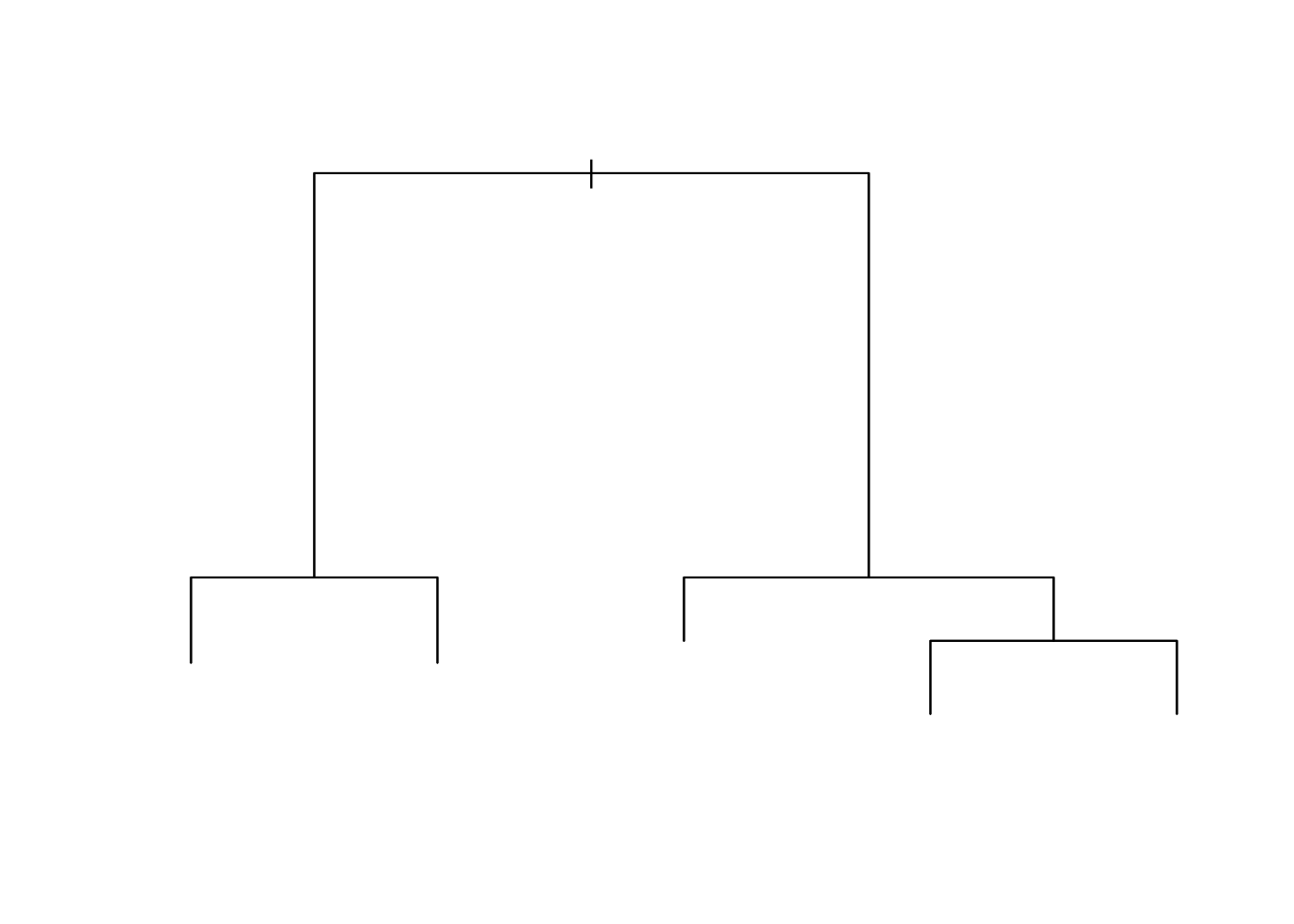
As you can see when you plot this, this only plots the empty decision tree, as such you will need to add a text() function separately.
- Repeat plotting the outcome object of your decision tree, with in the next line adding the
text()function, with as inputyour_tree_modelandpretty = 0.
plot(tree_qual)
text(tree_qual, pretty = 0)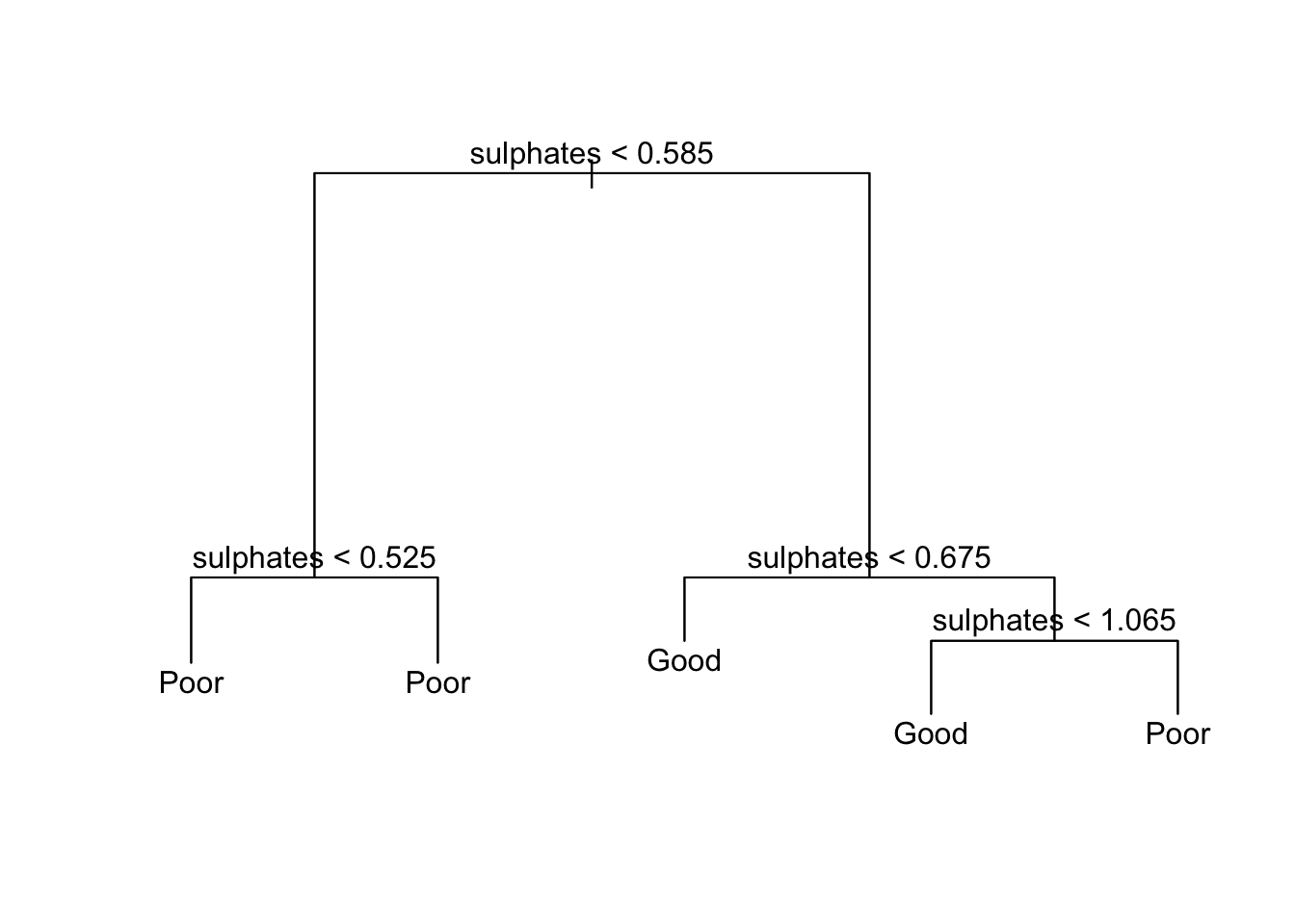
This now adds the text to the to the decision tree allowing it to be specified visually.
Although plotting the decision tree can be useful for displaying how a topic is split, it only goes some way to answering the research question presented. As such, additional steps are required to ensure that the tree is efficiently fitted.
Firstly, you can explore the layout of the current model using the summary() function. This displays the predictors used within the tree; the number of terminal nodes; the residual mean deviance and the distribution of the residuals.
- Using the
summary()function, examine the current decision tree, and report the number of terminal nodes and the residual mean deviance.
summary(tree_qual)##
## Classification tree:
## tree(formula = bin_qual ~ fixed_acidity + residual_sugar + pH +
## sulphates, data = wine_train)
## Variables actually used in tree construction:
## [1] "sulphates"
## Number of terminal nodes: 5
## Residual mean deviance: 1.235 = 1575 / 1275
## Misclassification error rate: 0.3336 = 427 / 1280Part 2: to be completed during the lab
Classification trees continued
Assessing accuracy and pruning of classification trees
During the homework part, you have fitted a classification tree on the Red Wine Quality dataset. In this first part during the lab, we will continue with your fitted tree, and inspect its overall accuracy and improvement through pruning. To examine the overall accuracy of the model, you should determine the prediction accuracy both for the training and the validation set. Using the predicted and observed outcome values, we can construct a confusion matrix, similar to what we’ve done in week 5 on Classification methods.
So let us build a confusion matrix for the training subset. To begin, once more you need to calculate the predicted value under the model. However, now you need to specify that you want to use type = "class"; before forming a table between the predicted values and the actual values. As shown below
# Create the predictions
    yhat_wine_train <- predict(tree_qual, newdata = wine_train, type = "class")

# Obtain the observed outcomes of the training data
    qual_train <- wine_train[, "bin_qual"]

# Create the cross table:
    tab_wine_train <- table(yhat_wine_train, qual_train)
    tab_wine_train
## qual_train
## yhat_wine_train Good Poor
## Good 511 254
## Poor 173 342The obtained confusion matrix indicates the frequency of a wine predicted as good while it is actually good or poor, and the frequency of wine predicted as poor while actually being good or poor. The frequencies in the confusion matrix are used to determine the accuracy through the formula:
Accuracy = (True Positive Predictions + True False Predictions) / total number of items
# Calculate Accuracy accordingly:
  accuracy_wine_train <- (tab_wine_train[1] + tab_wine_train[4]) / (tab_wine_train[1] +    tab_wine_train[2] + tab_wine_train[3] + tab_wine_train[4])

  accuracy_wine_train
## [1] 0.6664062From this, you can see that this model has an accuracy of around 67% meaning that 67% of the time, it is able to correctly predict from the predictors whether a wine will be of good or poor quality.
- Using this format, create a confusion matrix for the validation subset, and calculate the associated accuracy.
Hint: you can obtain the predicted outcomes for the validation set using predict(your_tree_model, newdata = wine_valid, type = "class") and you can extract the observed outcomes of the validation data using wine_valid[, "bin_qual"].
# Create the predictions
    yhat_qual_valid <- predict(tree_qual, newdata = wine_valid, type = "class")

# Obtain the observed outcomes of the validation data
    qual_valid <- wine_valid[, "bin_qual"]

# Create the cross table:
    tab_qual_valid <- table(yhat_qual_valid, qual_valid)
    tab_qual_valid
## qual_valid
## yhat_qual_valid Good Poor
## Good 126 62
## Poor 45 86# Calculate Accuracy accordingly:
accuracy_qual_valid <- (tab_qual_valid[1] + tab_qual_valid[4]) / tab_qual_valid[1] + tab_qual_valid[2] + tab_qual_valid[3] + tab_qual_valid[4]
accuracy_qual_valid## [1] 194.6825Now, let’s evaluate whether pruning this tree may lead to an improved tree. For this, you use the function cv.tree(). This runs the tree repeatedly, at each step reducing the number of terminal nodes to determine how this impacts the deviation of the data. You will need to use the argument FUN = prune.misclass to indicate we are looking at a classification tree.
- Run the model through the
cv.tree()function and examine the outcome using theplot()function using the code below.
# Determine the cv.tree
  cv_quality <- cv.tree(your_tree_model, FUN=prune.misclass)

# Plot the size vs dev
  plot(cv_quality$size, cv_quality$dev, type = 'b')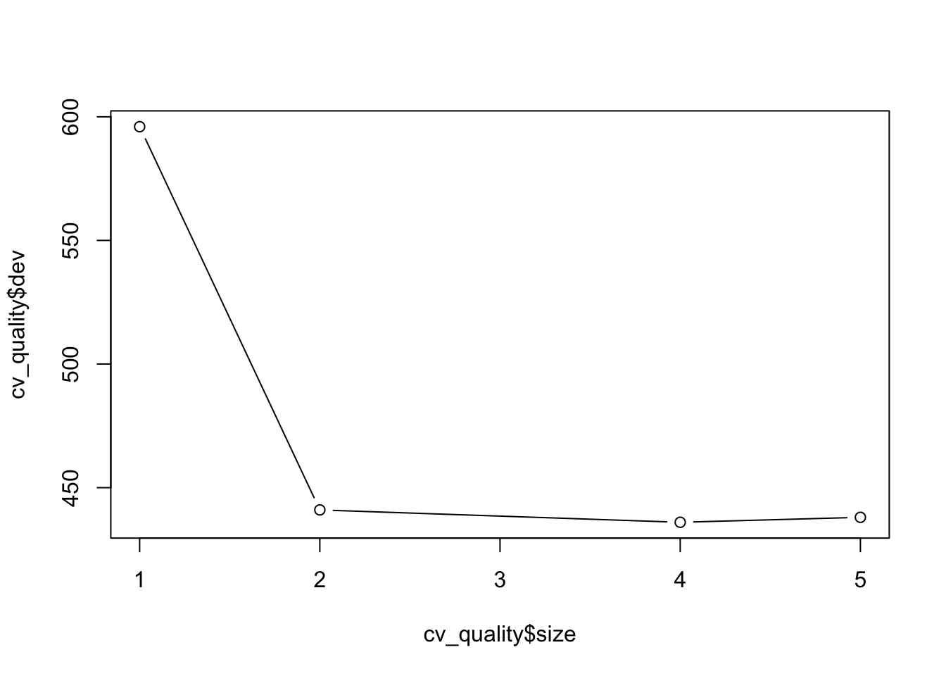
When you have run this code, you should observe a graph, which plots the size (the amount of nodes) against the dev (cross-validation error rate). This indicates how this error rate changes depending on how many nodes are used. In this case you should be able to observe a steep drop in dev between 1 and 2, before it slowing down from 2 to 5 (the maximum number of nodes used). If you would further like to inspect this, you could compare the accuracy (obtained from the confusion matrices) between these different models, to see which is best fitting. In order to prune the decision tree, you simply use the function prune.misclass(), providing both the model and best = number of nodes as your arguments.
Note that in the same way as growing classification trees, you can use the function tree() to grow regression trees. Regarding the input of the function tree() nothing has to be changed: the function detects whether the outcome variable is categorical as seen in the above example, applying classification trees, or continuous, applying regression trees. Differences arise at evaluating the decision tree (inspecting the confusion matrix and accuracy for classification trees or inspecting the MSE for regression trees) and at pruning. To prune a classification tree, you use the function prune.mislcass(), while for regression trees the function prune.tree() is used.
Bagging and Random Forests
When examining the techniques of Bagging and Random Forests, it is important to remember that Bagging is simply a specialized case of Random Forests where the number of predictors randomly sampled as candidates at each split is equal to the number of predictors available, and the number of considered splits is equal to the number of predictors.
So for example, if you were looking to predict the quality of wine (as we have done during the classification tree section), based upon the predictors fixed acidity (fixed_acidity), citric acid (citric_acid), residual sugars (residual_sugar), pH (pH), total sulfur dioxide content (total_sulfar_dioxide), density (density) and alcohol (alcohol) content. If we were to undergo the bagging process we would limit the number of splits within the analysis to 7, whereas within random forest it could be any number of values you choose.
As such, the process of doing Bagging or Random Forests is similar, and both will be covered. When using these methods we get an additional measure for model accuracy in addition to the MSE: the out of bag (OOB) estimator. Also, we can use the variable importance measure to inspect which predictors in our model contribute most to accurately predicting our outcome.
Note that we will focus on a classification example, while the ISLR textbook focuses on a regression tree example.
Bagging
Both Bagging and Random Forest are based around the function randomForest() from the randomForest package. The function requires the following components:
randomForest(formula = ???,       # Tree Formula
             data = ???,          # Data Set
             subset = ???,        # How the data set should be subsetted
             mtry = ???,          # Number of predictors to be considered for each split
             importance = TRUE,   # The Variable importance estimator
             ntree = ???)         # The number of trees within the random forest
In the case of bagging, the argument mtry should be set to the quantity of the predictors used within the model.
- Create a bagging model for the research question: can we predict quality of wine
bin_qual, byfixed_acidity,citric_acid,residual_sugar,pH,total_sulfur_dioxide,densityandalcoholand inspect the output. Omitntreefrom the functions input for now.
  bag_qual <- randomForest(formula = bin_qual ~ fixed_acidity + citric_acid + residual_sugar +
                             pH + total_sulfur_dioxide + density + alcohol,
                           data = wine_train,
                           mtry = 7,
                           importance = TRUE)
  bag_qual
##
## Call:
## randomForest(formula = bin_qual ~ fixed_acidity + citric_acid + residual_sugar + pH + total_sulfur_dioxide + density + alcohol, data = wine_train, mtry = 7, importance = TRUE)
## Type of random forest: classification
## Number of trees: 500
## No. of variables tried at each split: 7
##
## OOB estimate of error rate: 21.56%
## Confusion matrix:
## Good Poor class.error
## Good 551 133 0.1944444
## Poor 143 453 0.2399329How do we interpret the output of this classification example? From this output, you can observe several different components. Firstly, you should be able to observe that it recognizes that this is a Classification forest, with 500 trees (the default setting for number of trees) and 7 variables tried at each split. In addition, the OOB estimate is provided in the output as well as a classification confusion matrix.
Let us examine the the accuracy level of our initial model, and compare it to the accuracy of models with a varying number of trees used.
- Calculate the accuracy of the bagged forest you just fitted
acc_bag_qual <- (bag_qual$confusion[1,1] + bag_qual$confusion[2,2]) / (bag_qual$confusion[1,1] + bag_qual$confusion[1,2] + bag_qual$confusion[2,1] + bag_qual$confusion[2,2])Now let’s have a look at the Out of Bag (OOB) estimator of error rate. The OOB estimator of the error rate is provided automatically with the latest version of randomForest(), and can be used as a valid estimator of the test error of the model. In the OOB estimator of the error rate, the left out data at each bootstrapped sample (hence, Out of Bag) is used as the validation set. That is, the response for each observation is predicted using each of the trees in which that observation was OOB. This score, like other indicates of accuracy deviation, you will want as low as possible, since it indicates the error rate.
- Inspect the OOB scores of the bagged forest you fitted.
# 500 Trees = 22.46%- Fit two additional models, in which you set the number of trees used to 100 and 10000, and inspect the OOB scores. Which has the highest and lowest OOB estimate?
bag_qual_100 <- randomForest(formula = bin_qual ~ fixed_acidity + citric_acid + residual_sugar +
                             pH + total_sulfur_dioxide + density + alcohol,
                           data = wine_train,
                           mtry = 7,
                           importance = TRUE,
                           ntree = 100)

bag_qual_10000 <- randomForest(formula = bin_qual ~ fixed_acidity + citric_acid + residual_sugar +
                             pH + total_sulfur_dioxide + density + alcohol,
                           data = wine_train,
                           mtry = 7,
                           importance = TRUE,
                           ntree = 10000)

bag_qual_100
##
## Call:
## randomForest(formula = bin_qual ~ fixed_acidity + citric_acid + residual_sugar + pH + total_sulfur_dioxide + density + alcohol, data = wine_train, mtry = 7, importance = TRUE, ntree = 100)
## Type of random forest: classification
## Number of trees: 100
## No. of variables tried at each split: 7
##
## OOB estimate of error rate: 21.41%
## Confusion matrix:
## Good Poor class.error
## Good 549 135 0.1973684
## Poor 139 457 0.2332215bag_qual_10000##
## Call:
## randomForest(formula = bin_qual ~ fixed_acidity + citric_acid + residual_sugar + pH + total_sulfur_dioxide + density + alcohol, data = wine_train, mtry = 7, importance = TRUE, ntree = 10000)
## Type of random forest: classification
## Number of trees: 10000
## No. of variables tried at each split: 7
##
## OOB estimate of error rate: 21.17%
## Confusion matrix:
## Good Poor class.error
## Good 556 128 0.1871345
## Poor 143 453 0.2399329# OOB estimates:
# 10 Trees = 22.3%
# 10000 Trees = 21.6%
# Note that these values will fluctuate somewhatRandom Forests
The main difference between Bagging and Random Forests is that the number of predictors randomly sampled as candidates at each split is not equal to the number of predictors available. In this case, typically (by default from the randomForest() function), they determine mtry to be 1/3 the number of available predictors for regression trees and the square root of the number of available predictors for classification trees.
- Using the
randomForest()function, construct a random forest model usingmtry = 3andntree = 500.
  for_qual_3 <- randomForest(formula = bin_qual ~ fixed_acidity + citric_acid + residual_sugar +
                             pH + total_sulfur_dioxide + density + alcohol,
                           data = wine_train,
                           mtry = 3,
                           importance = TRUE,
ntree = 500)- Inspect fitted random forest model and the corresponding the OOB estimate of the random forest model and compare to the OOB estimate of the bagged forest model with
ntree = 500.
for_qual_3##
## Call:
## randomForest(formula = bin_qual ~ fixed_acidity + citric_acid + residual_sugar + pH + total_sulfur_dioxide + density + alcohol, data = wine_train, mtry = 3, importance = TRUE, ntree = 500)
## Type of random forest: classification
## Number of trees: 500
## No. of variables tried at each split: 3
##
## OOB estimate of error rate: 21.02%
## Confusion matrix:
## Good Poor class.error
## Good 560 124 0.1812865
## Poor 145 451 0.2432886# OOB random forest:
# 22.6 % Variable importance
The final (optional) part of this practical will look into how to actually interpret Random Forests, using the Variable Importance Measure. As you have probably worked out from section so far, physically representing these forests is incredibly difficult and harder to interpret them, in comparison to solo trees. As such, although creating random forests improves the prediction accuracy of a model, this is at the expense of interpretability. Therefore, to understand the role of different predictors within the forests as a whole it is important to examine the measure of Variable Importance.
Overall, when looking at Regression Trees, this Variable Importance measure is calculated using the residual sum of squares (RSS) and via the Gini Index for classification trees. Conveniently, the correct version will be determined by the randomForest() function, as it can recognize whether you are creating a regression or classification tree forest.
In order to call this measure, we simply need to call the model into the function importance(). Within our case (looking at a classification forest) this will produce four columns, the binary outcome (Good/Poor) in addition to the Mean Decrease in Accuracy and the Mean Decrease in Gini Index. This is by contrast to those which you will find when examining Regression trees, examples of which can be found in ISLR Section 8.3.3.
In order to best interpret these findings, it is possible to plot, how important each predictor is using the function varImpPlot(). This will produce a sorted plot which will show the most to least important variables.
- Using your random forest model, examine the importance of the predictors using
importance()and usevarImpPlot()to plot the result. Which predictor is most important to predict the quality of Wine?
  # 1. Run the importance to get a rough idea of which predictors are most important
  importance(for_qual_3)
## Good Poor MeanDecreaseAccuracy MeanDecreaseGini
## fixed_acidity 24.12648 20.50581 36.78868 71.67600
## citric_acid 26.92849 28.40715 40.38459 72.19014
## residual_sugar 24.57684 21.59432 34.41618 59.80545
## pH 24.38166 21.21343 34.49138 71.89639
## total_sulfur_dioxide 41.02922 35.46611 53.45830 105.92436
## density 30.49423 20.02408 41.06932 92.80302
## alcohol 64.64370 65.67504 92.94490 162.10072 # 2_ Run for_qual_3 through varImpPlot() to plot this importance
varImpPlot(for_qual_3)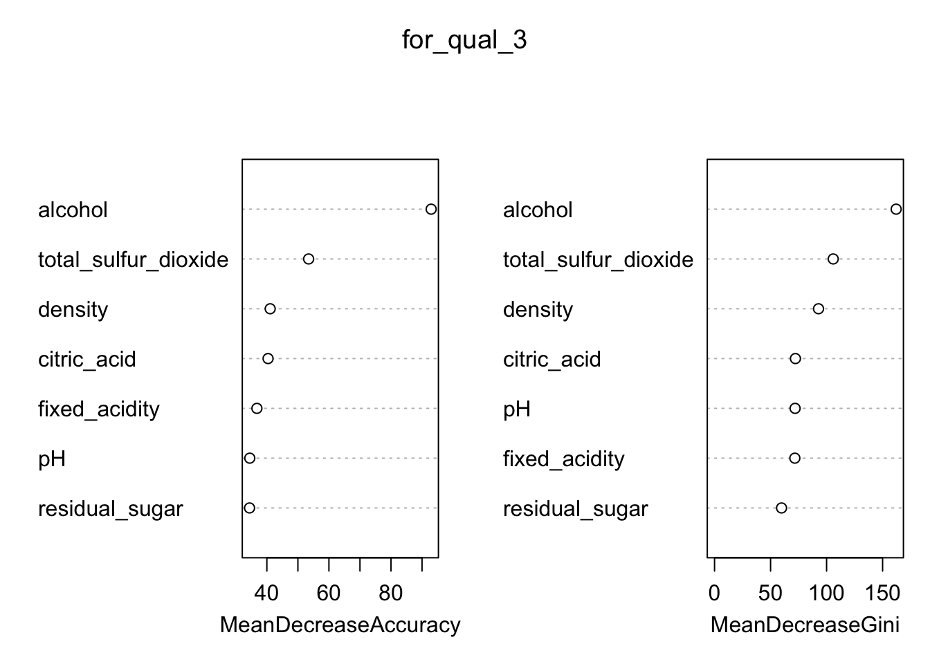
  # The alcohol content of the wine is seen as the most important predictor
    # As to whether the wine is good or bad quality